Quick-start Guide

This guide is walkthrough for the Dprofiler from start to finish.

Getting Started

First off, we need to install R package of Dprofiler from GitHub:

if (!requireNamespace("remotes", quietly=TRUE))
  install.packages("remotes")
remotes::install_github("UMMS-Biocore/dprofiler")

One you have installed the R package, you can call these R commands:

library(dprofiler)
startDprofiler()

Once you’ve made your way to the website, or you have a local instance of Dprofiler running, you will be greeted with data loading section:

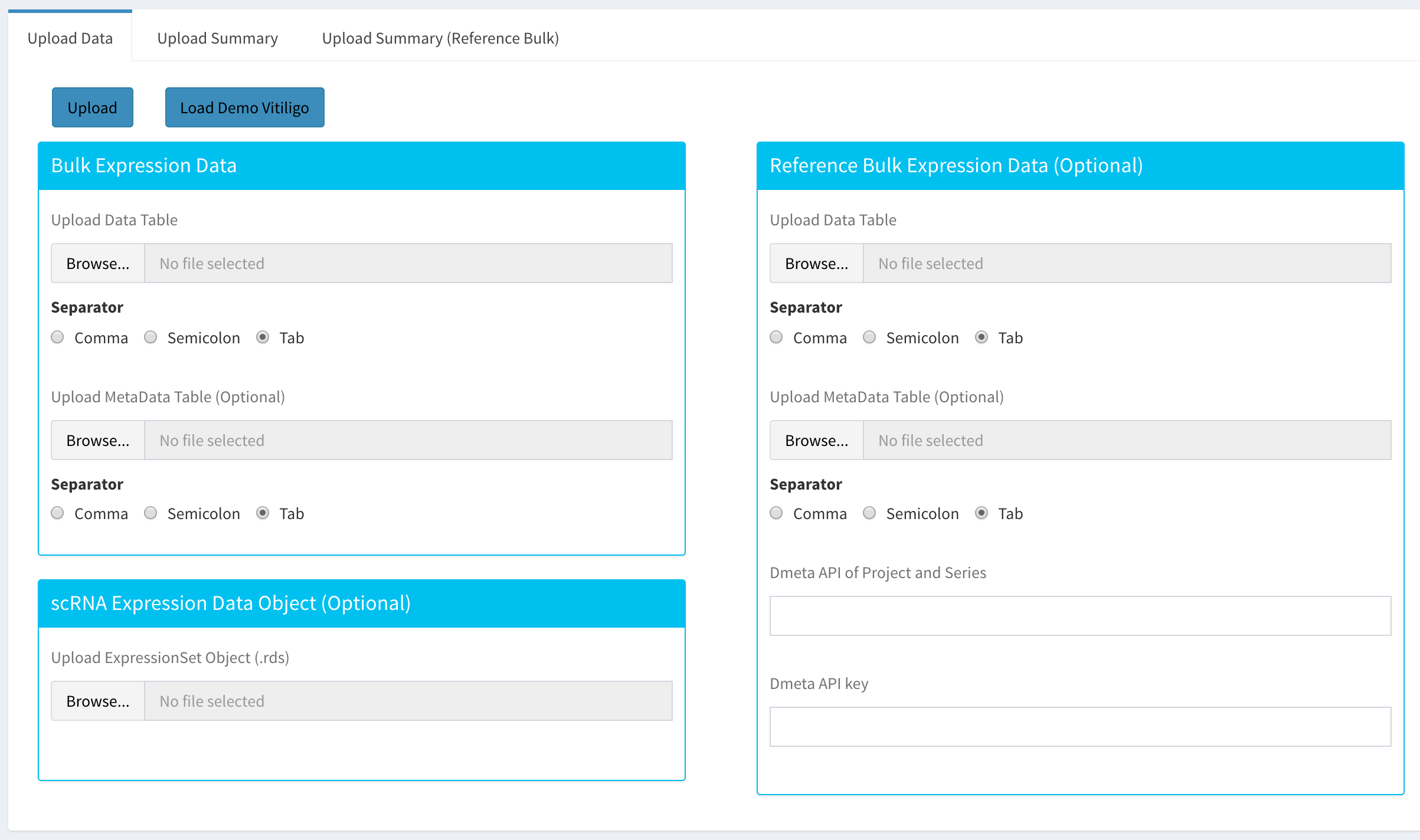
To begin the analysis, you need to upload your data files (comma or semicolon separated, i.e. “.csv”, or tab separated, i.e. “.tsv”, format) to be analyzed and choose appropriate separator for the file (comma, semicolon or tab).

There are three types input data in Dprofiler. These are:

• Bulk Expression Data: used for profiling samples within and establish homogeneous reference profiles.

• scRNA Expression Data Object: used for deconvoluting Bulk RNA data and infering cellular compositions of these bulk samples.

• Reference Bulk Expression Data: used for comparative profiling of the Bulk data set using reference phenotypic profiles of reference bulk data set(s).

If you do not have a dataset to upload, you can use the built in demo data file by clicking on the ‘Load Demo Vitiligo’ button that loads a case study. To view the entire demo data file, you can download.

• PRJNA554241: a bulk RNA-Seq count data of lesional and non-lesional vitiligo skin samples processed by the RNA-Seq pipeline of DolphinNext .

• scVitiligo: a reference scRNA-Seq count data of lesional and non-lesional vitiligo skin samples.

• GSE65127: an external bulk microarray data of vitiligo skin samples where the gene set is union of differentially expressed genes across four conditions: healthy, lesional, non-lesional and peri-lesional.

Otherwise, you can start uploading your own data given instructions below.

Input for Bulk Expression Data

For both submitted Bulk and Reference Bulk expression data, you need to upload your data files (comma or semicolon separated, i.e. “.csv”, or tab separated, i.e. “.tsv”, format) to be analyzed and choose appropriate separator for the file (comma, semicolon or tab). However, for scRNA data set, the user should provide an ExpressionSet object. In addition, users may connect to DolphinMeta using their credentials to import reference bulk expression data from any Dmeta project.

An example structure of the count data files are shown below:

gene	P39_NL	P39_L	P33_NL	P33_L	P22_NL	P22_L	P19_NL	P19_L	P65_NL	P65_L
A1BG	46	29	104	27	42	17	65	101	27	32
A1BG-AS1	27	18	48	13	10	3	39	54	23	24
A1CF	5	0	38	15	2	0	4	7	0	3

In addition to the count data file; you might need to upload metadata files to correct for batch effects or any other normalizing conditions you might want to address that might be within your results. To handle for these conditions, simply create a metadata file by using the example table at below. Metadata file also simplifies condition selection for complex data. The columns you define in this file can be selected in condition selection page. Make sure you have defined two conditions per column. If there are more than two conditions in a column, those can be defined empty. Please note that, if your data is not complex, metadata file is optional, you don’t need to upload.

In the example below, the “patient” column may serve as a batch or a normalizing condition.

sample	patient	treatment
P39_NL	P39	NL
P39_L	P39	L
P33_NL	P33	NL
P33_L	P33	L
P22_NL	P22	NL
P22_L	P22	L
P19_NL	P19	NL
P19_L	P19	L
P65_NL	P65	NL
P65_L	P65	L

Metadata file can be formatted with comma, semicolon or tab separators similar to count data files. These files used to establish different batch effects for multiple conditions. You can have as many conditions as you may require, as long as all of the samples are present.

Alternatively, you can connect to your DolphinMeta (Dmeta) account using your access token and import external expression profiles and associated metadata.

Input for scRNA Expression Data

However, for scRNA data set, the user should provide an .rds file containing an ExpressionSet object whose metadata (pData(You Expression Set Object)) should include the following variables or columns:”,

• (i) sample associated to each barcode

• (ii) total UMI counts of each barcode

• (iii) cell annotation or label of each barcodes

• (iv) other categorical and numerical variables relavant to barcodes

Once the count data and metadata files have been loaded in Dprofiler, you can click upload button to visualize your data as shown below:

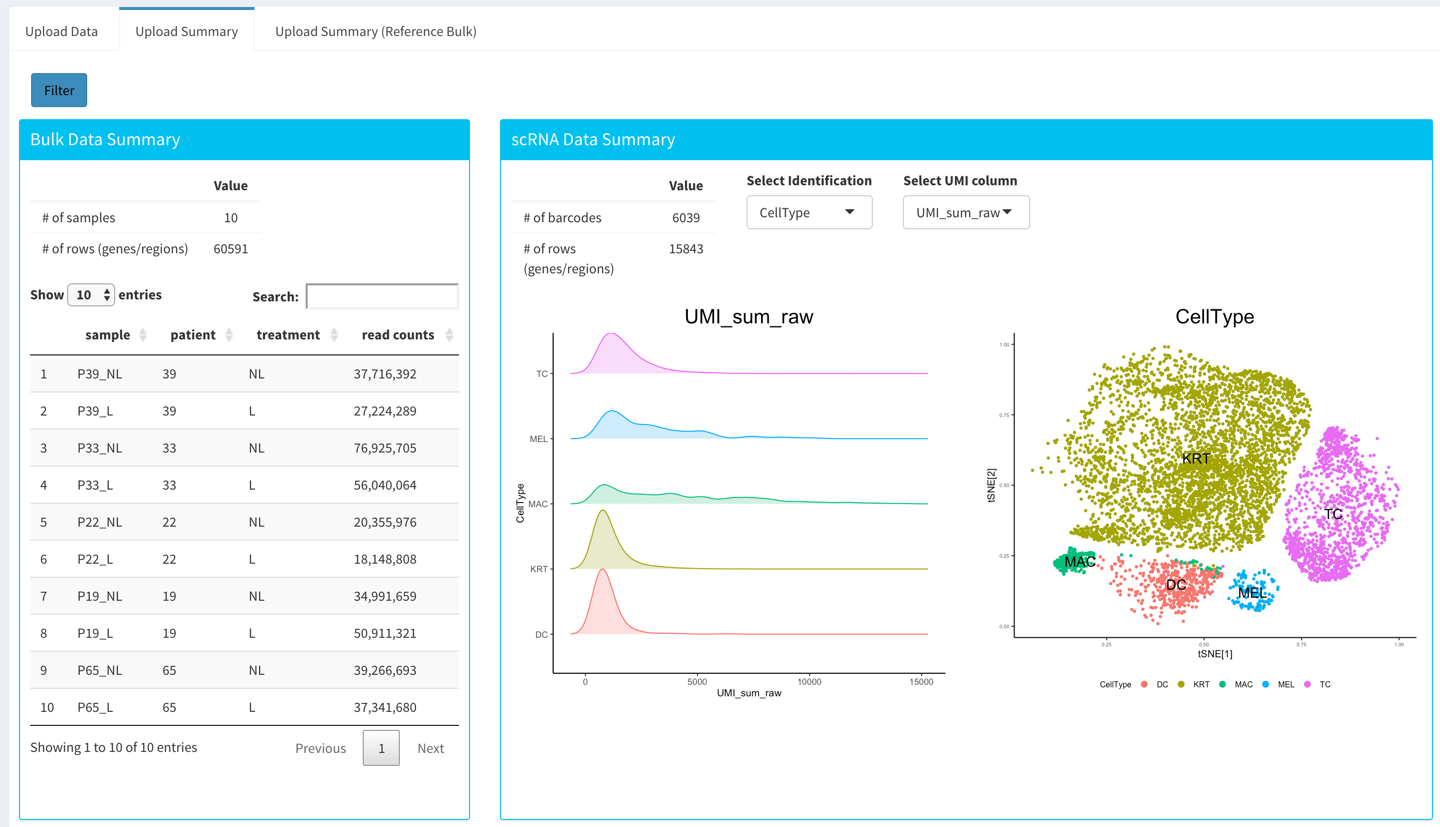
You have the option to search samples or other terms within submitted or reference bulk Expression data sets, and you also have the option to visualize the t-SNE and other numeric measures of your barcodes within the uploaded scRNA expression data object.

After reviewing your uploaded data in “Upload Summary” panels, and if specified the metadata file containing your batch correction fields, you then have the option to filter low counts and conduct batch effect correction prior to your analysis. Alternatively, you may skip these steps and directly continue with Computational Profiling analysis.

Data analysis steps such as “Low Count Filtering”, “Batch Effect Correction”, “Computational Profiling” are only applicable to the submitted bulk expression data, and other submitted reference scRNA and bulk RNA datasets are used for referential purposes and assumed to be already filtered and analyzed before submission.

Low Count Filtering

In this section, you can simultaneously visualize the changes of your submitted bulk RNA expression data while filtering out the low count genes. Choose your filtration criteria from Filtering Methods box which is located just center of the screen. Three methods are available to be used:

• Max: Filters out genes where maximum count for each gene across all samples are less than defined threshold.

• Mean: Filters out genes where mean count for each gene are less than defined threshold.

• CPM: First, counts per million (CPM) is calculated as the raw counts divided by the library sizes and multiplied by one million. Then it filters out genes where at least defined number of samples is less than defined CPM threshold.

After selection of filtering methods and entering threshold value, you can proceed by clicking Filter button which is located just bottom part of the Filtering Methods box. On the right part of the screen, your filtered dataset will be visualized for comparison as shown at figure below.

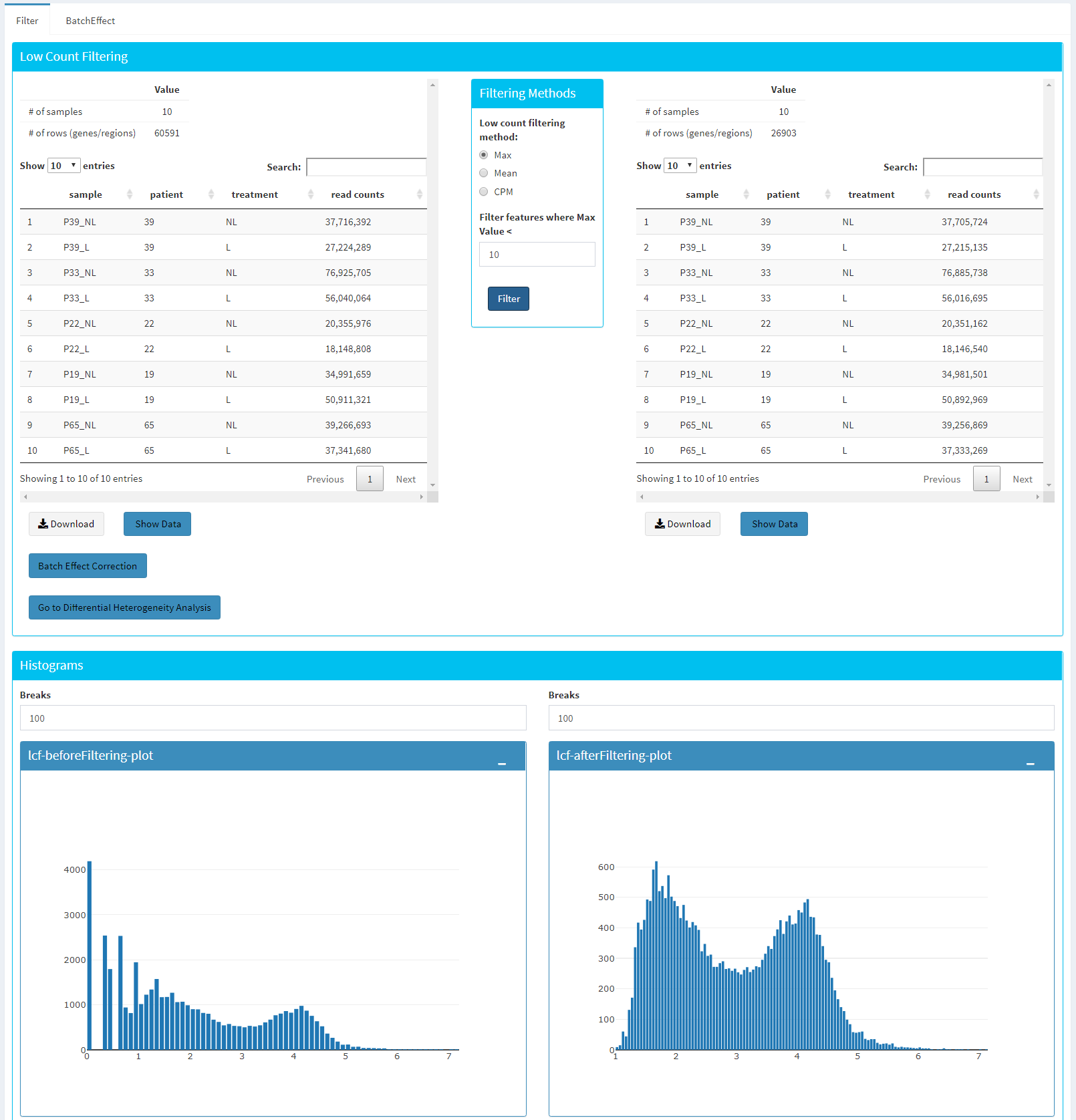
You can easily compare following features, before and after filtering:

• Number of genes/regions.

• Read counts for each sample.

• Overall histogram of the dataset.

• gene/region vs samples data

Important

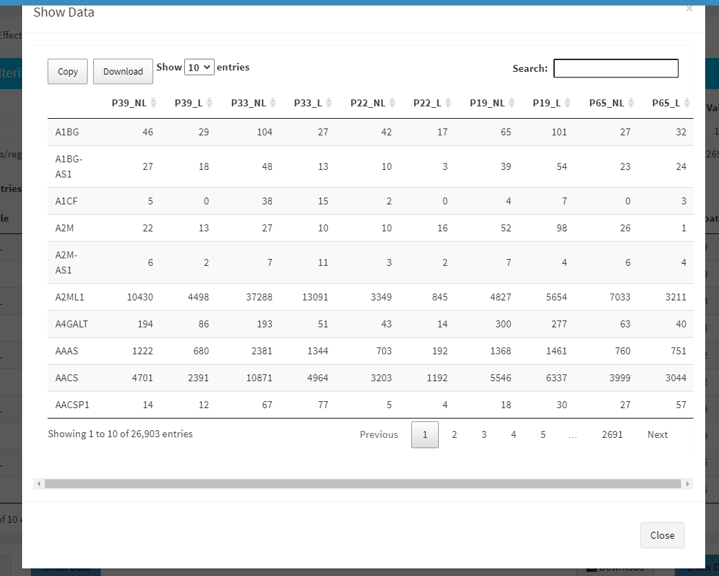
To investigate the gene/region vs samples data in detail as shown at below, you may click the Show Data button, located bottom part of the data tables. Alternatively, you may download all filtered data by clicking Download button which located next to Show Data button.

Afterwards, you may continue your analysis with Batch Effect Correction or directly jump to Computational Profiling of your dataset.

Batch Effect Correction and Normalization

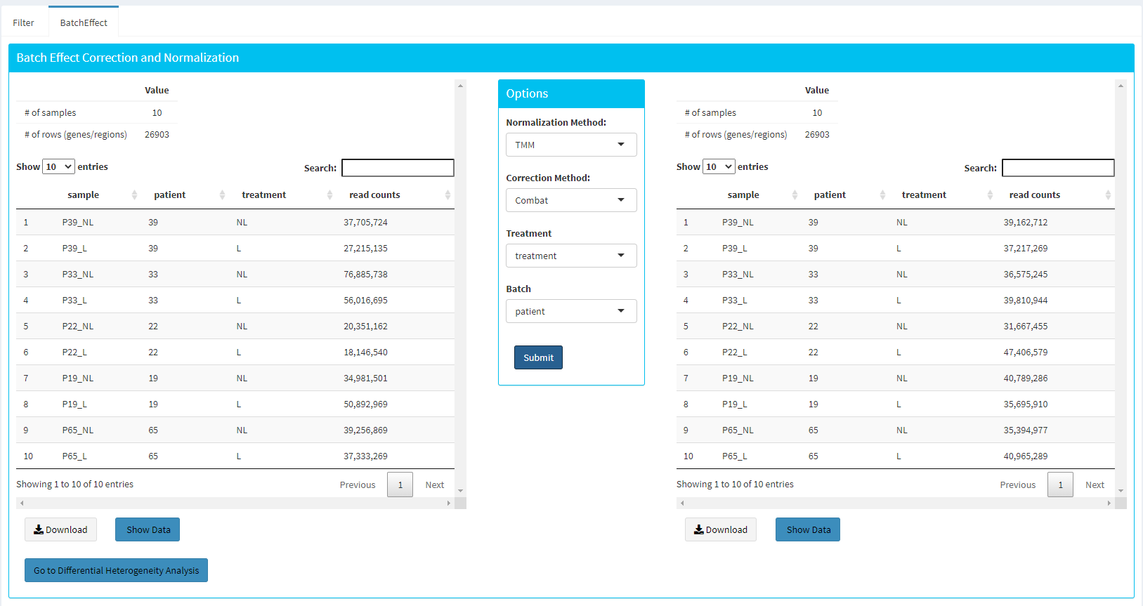
If specified metadata file containing your batch correction fields, then you have the option to conduct batch effect correction prior to your analysis. By adjusting parameters of Options box, you can investigate your character of your dataset. These parameters of the options box are explained as following:

• Normalization Method: Dprofiler allows performing normalization prior the batch effect correction. You may choose your normalization method (among MRN (Median Ratio Normalization), TMM (Trimmed Mean of M-values), RLE (Relative Log Expression) and upperquartile), or skip this step by choosing none for this item.

• Correction Method: Dprofiler uses ComBat (part of the SVA bioconductor package) or Harman to adjust for possible batch effect or conditional biases.

• Treatment: Please select the column that is specified in metadata file for phenotypic comparisons, such as cancer vs control.

• Batch: Please select the column name in metadata file which differentiate the batches.

Upon clicking submit button, comparison tables and plots will be created on the right part of the screen as shown below.

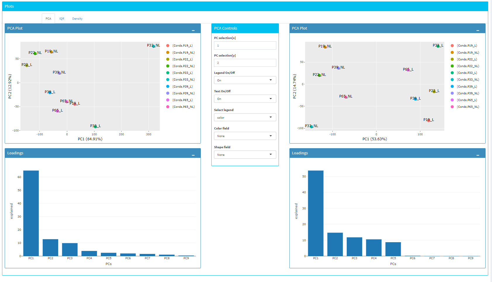
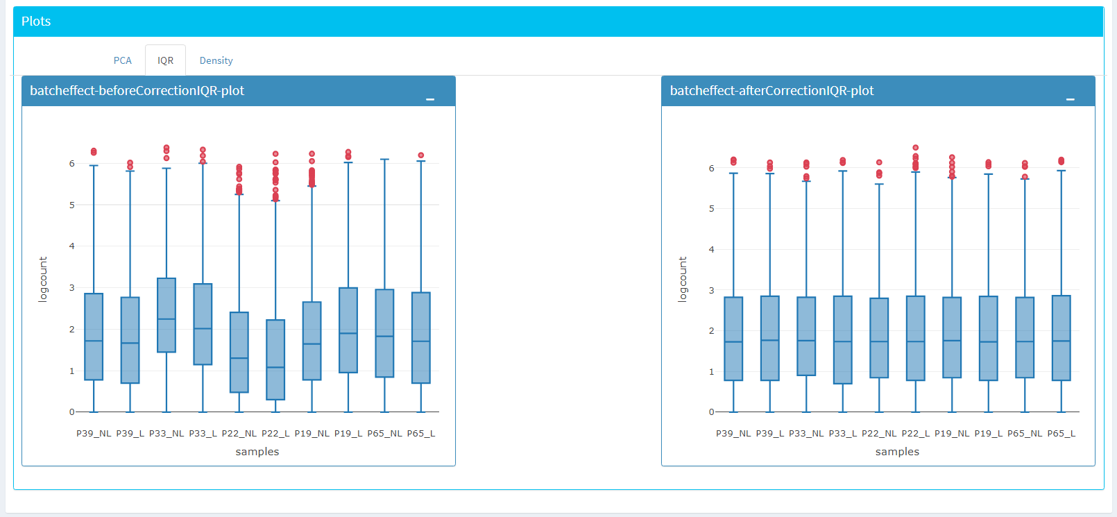
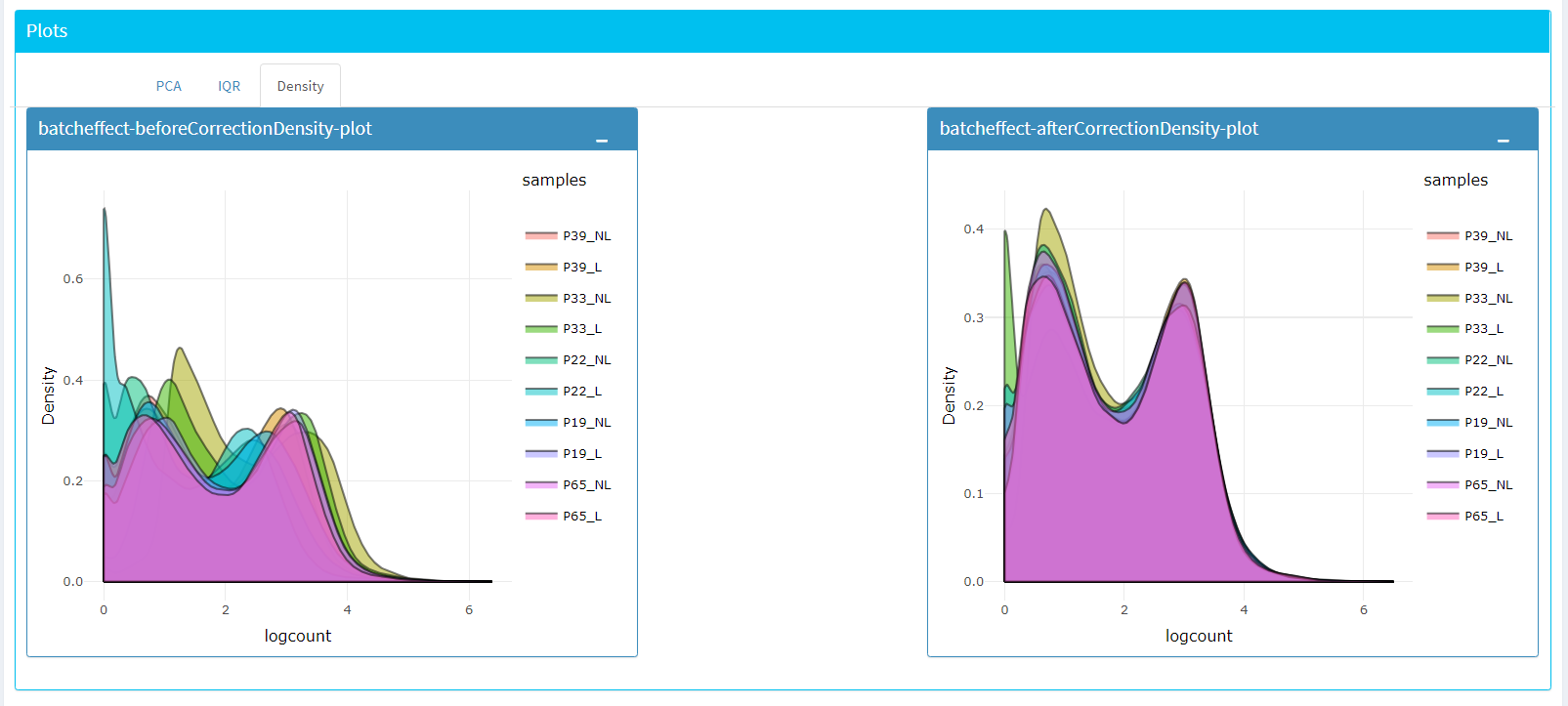
You can investigate the changes on the data by comparing following features:

• Read counts for each sample.

• PCA, IQR and Density plot of the dataset.

• Gene/region vs samples data

Tip

You can investigate the gene/region vs samples data in detail by clicking the Show Data button, or download all corrected data by clicking Download button.

Since we have completed batch effect correction and normalization step, we can continue with ‘Go to Computational Profiling’. This takes you to page where computational profiling is conducted with popular DE analysis methods like DESeq2, EdgeR or Limma.

Computational Profiling

The first option, ‘Go to Computational Profiling’, takes you to the next step where an iterative differential expression analysis and scoring of samples takes place.

• Sample Selection: In order to run the analysis, you first need to select the initial set of samples which will be compared or may be removed throughout the analysis. To do so, choose Select Meta box as treatment to simplify fill Condition 1 and Condition 2 based on the treatment column of the metadata as shown below.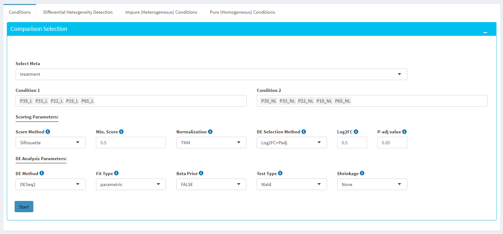

  

If you need to remove samples from a condition, simply select the sample you wish to remove and hit the delete/backspace key. In case, you need to add a sample to a condition you can click on one of the condition text boxes to bring up a list of samples and then click on the sample you wish to add from the list and it will be added to the textbox for that comparison.

Scoring Parameters: Two scoring methods are available for Dprofiler: Silhouette and NNLS-based.

• Silhouette method incorporates Spearman correlation measures between samples of the same phenotypic condition to estimate the magnitude of similarity between a particular sample and all other samples in the same group.

• NNLS-based method fits a non-negative regression model with a sample being the response and condition-specific (mean) expression profiles of conditions are input variables.

Both methods produce scores between (0,1) where lower values are associated with low membership score indicating that the sample is dissimilar to other samples in the same group/phenotype/condition. You can determine a threshold for low membership scores from the Min. Score option which is between (0,1). You can also determine additional criteria for selecting differentially expressed genes by DE Selection Method where additional options are provided to choose thresholds for parameters such as log2FC and P-adj value.

DE Parameters: Thera are three DE methods that are available for Dprofiler: DESeq2, EdgeR, and Limma. DESeq2 and EdgeR are designed to normalize count data from high-throughput sequencing assays such as RNA-Seq. On the other hand, Limma is a package to analyse of normalized or transformed data from microarray or RNA-Seq assays. Upon selecting any of three DE analysis methods, additional options will appear for parameters specific to the selected DE method.

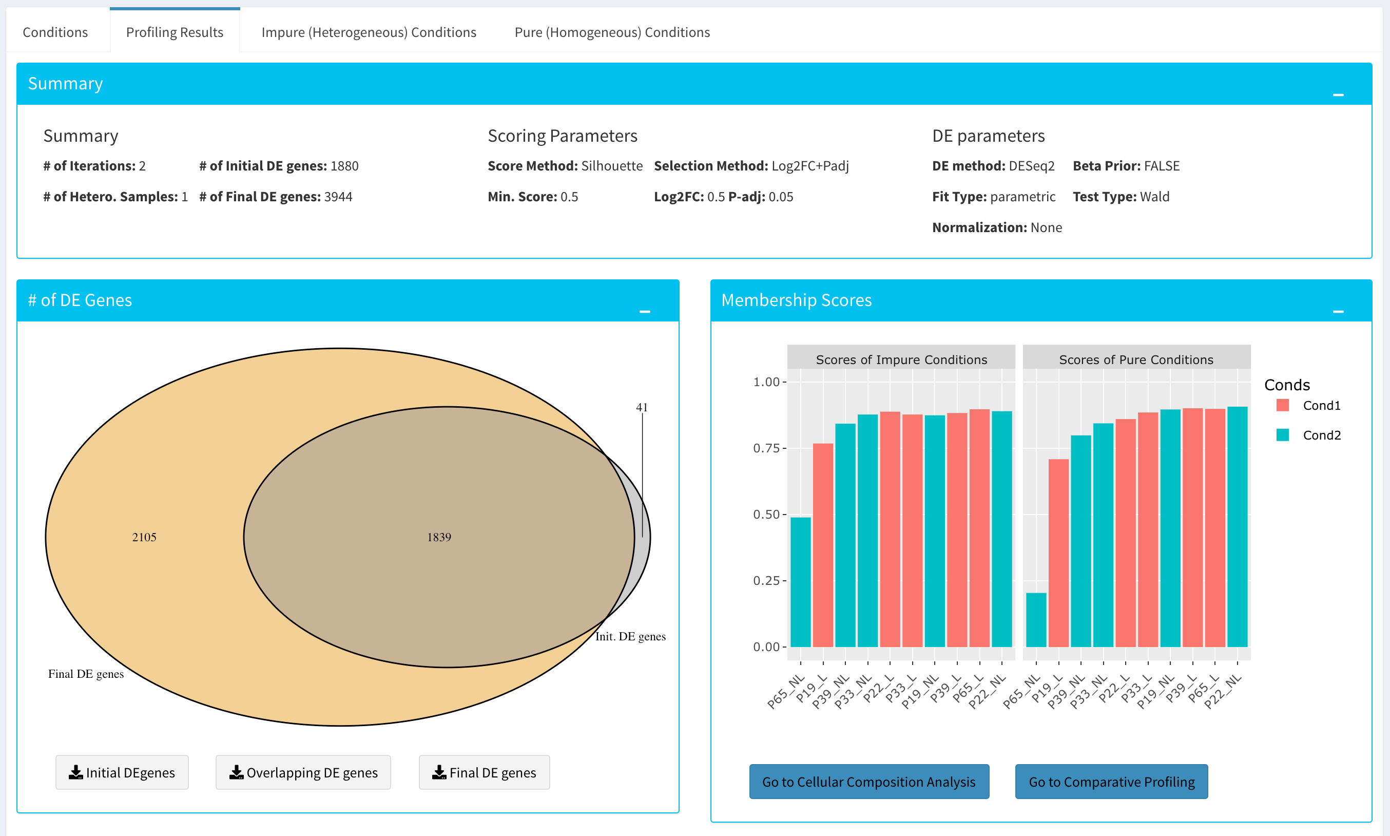
After clicking on the ‘start’ button, Dprofiler will analyze your selected comparison and conditions, and store the results into separate data tables. Upon finishing the Computational Profiling, three separate results panels will be produced:

• Profiling Results

• Impure (Heterogeneous) Conditions

• Pure (Homogeneous) Conditions

Upon finishing the Computational Profiling, the application will switch to “Profiling Results” panel showing results of the analysis. Differentially expressed genes of initial DE analysis and Final DE analysis are compared: that is the number of DE genes at the analysis at the first and last iteration are compared. The app also informs you about the parameters of the Scoring and DE analysis.

Additional information of initial and final DE genes can be found on plots below. Three Scatter Plots of initial and final genes, as well as the common genes in both list of DE genes will be plotted. You can switch to Volcano Plot and MA Plot by using Plot Type section at the left side of the Discover* menu. Since these plots are interactive, you can click to zoom button on the top of the graph and select the area you would like to zoom in by drawing a rectangle. Please see the plots at below:

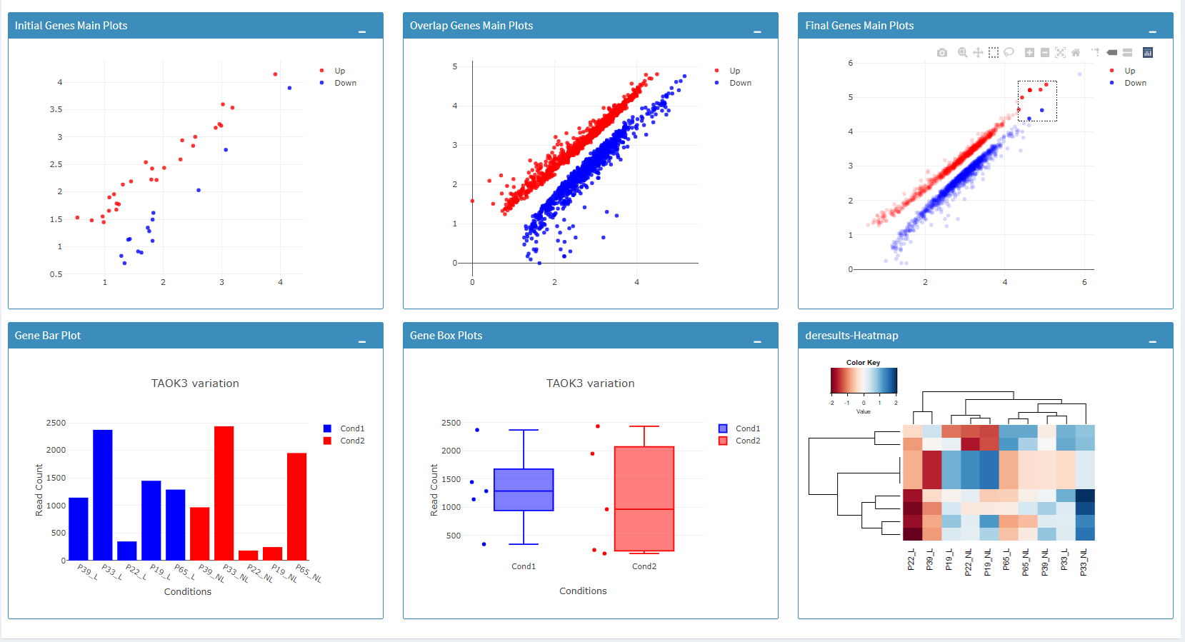
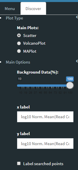
You can hover over the scatterplot points to display more information about the point selected. A few bargraphs will be generated for the user to view as soon as a scatterplot point is hovered over.

Tip

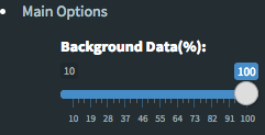
Please keep in mind that to increase the performance of the generating graph, by default 10% of non-significant(NS) genes are used to generate plots. You might show all NS genes by please click Main Options button and change Background Data(%) to 100% on the left sidebar.

Next, you can initiate a Cellular composition analysis using either the Homogeneouos, Heterogeneous conditions or marker genes, and deconvolute the Reference bulk expression data using the reference scRNA expression data by clicking “Go to Cellular Composition Analysis”. Or, you can click to “Go to Comparative Profiling” for the comparative analysis between the submitted bulk RNA expression and reference bulk RNA data.

But before that, you can take a look and investigate DE genes of either initial or Final DE analysis from remaining panels.

Impure and Pure Conditions

There are two more panels on the right of Profiling Results panel which take a closer look at initial and final DE genes of the conditions.

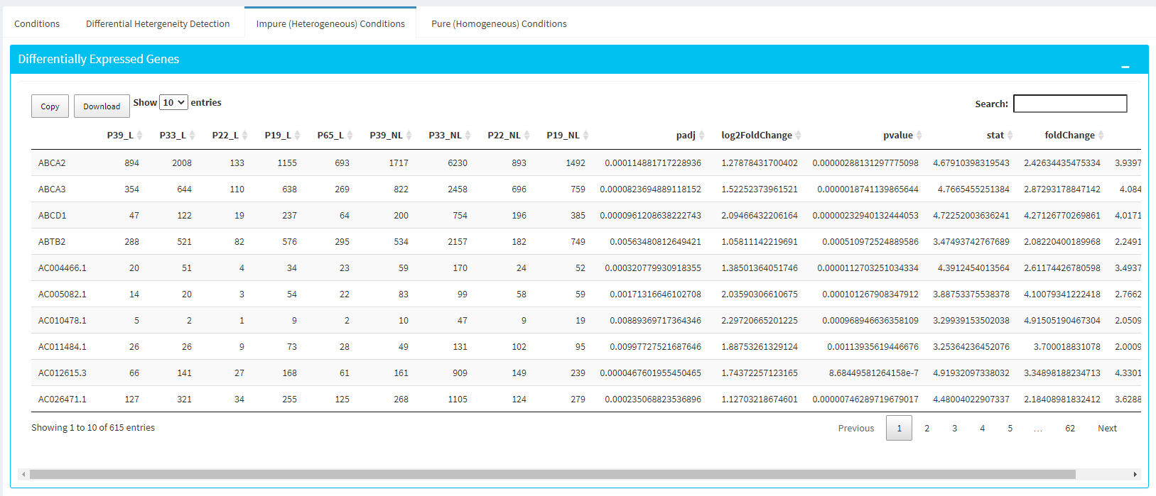
You can always download these results in CSV format by clicking the Download button. You can also download the plot or graphs by clicking on the download button at top of each plot or graph.

Cellular Composition Analysis

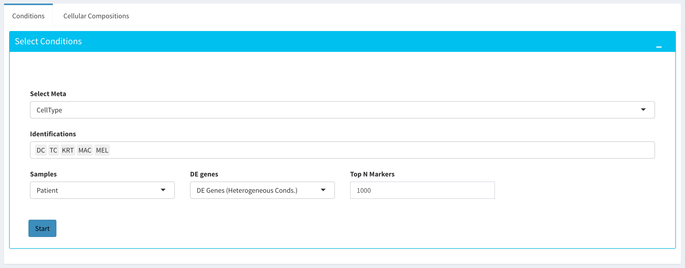
By using the “Cellular Comp. Analysis” tab, you can determine which idents (or identifications, categories) are to be used to deconvolute the submitted bulk expression data. You can also choose which of those cell types within each ident are to be used for the deconvolution as well. Then you can also decide whether DE genes of initial or final DE analysis are used to deconvolute the data. You should decide which column in the scRNA metadata that the samples are introduced, this is required by the MUSIC algorithm to give weight to genes that are less variant across different samples. You can also determine the set of genes to deconvolute bulk samples where you can either use DE genes of impure or pure conditions associated to the initial and final DE analysis, or you can use the marker genes of all selected cell types stored in fData(You scRNA Expression object).

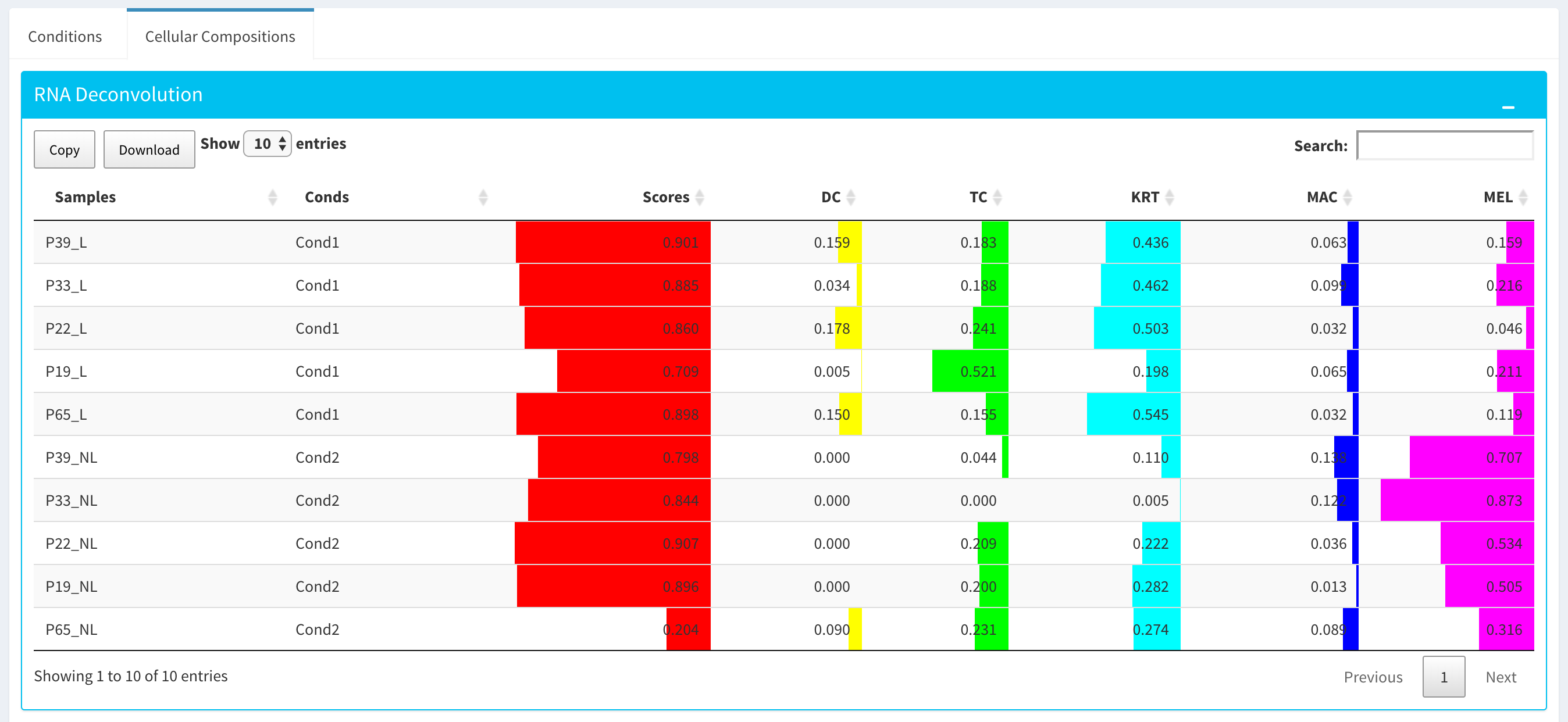
After clicking the “Start” button, the results will be given in the “Cellular Compositions” panel. Membership Scores and estimated cell type fractions are given for each sample where each box of the table are highlighted with respect to cell type.

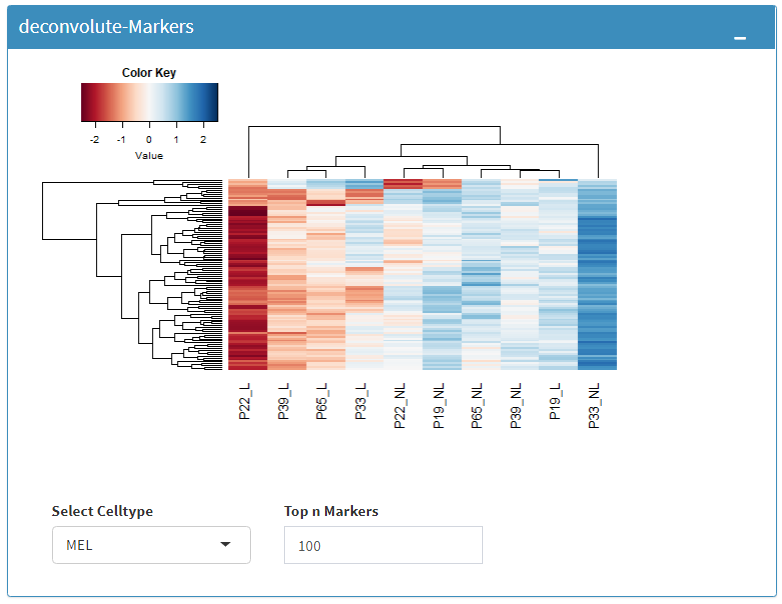
You can also visualize count data of Reference bulk expression data set with respect to cellular markers using interactive heatmaps.

Comparative Profiling

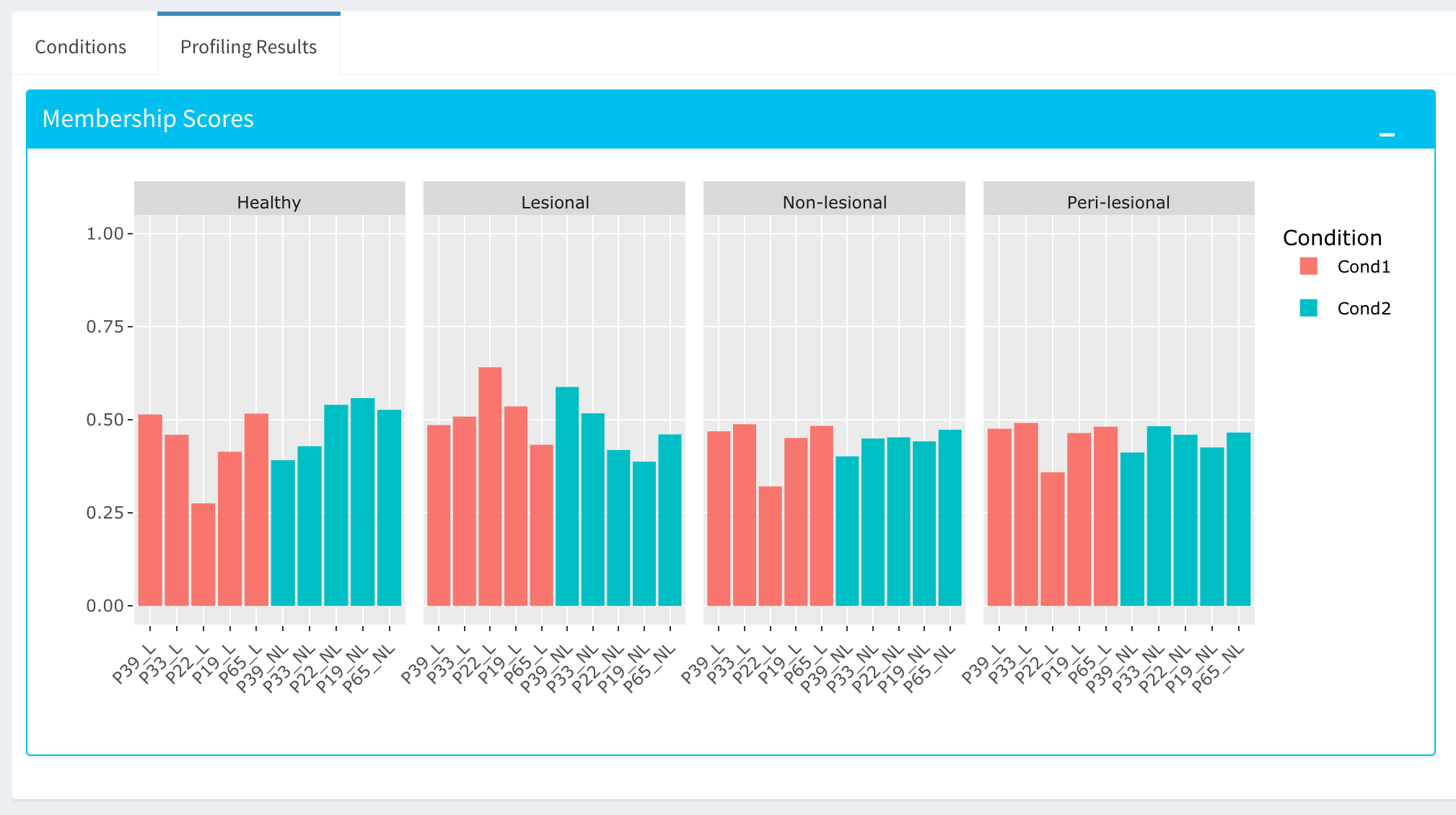
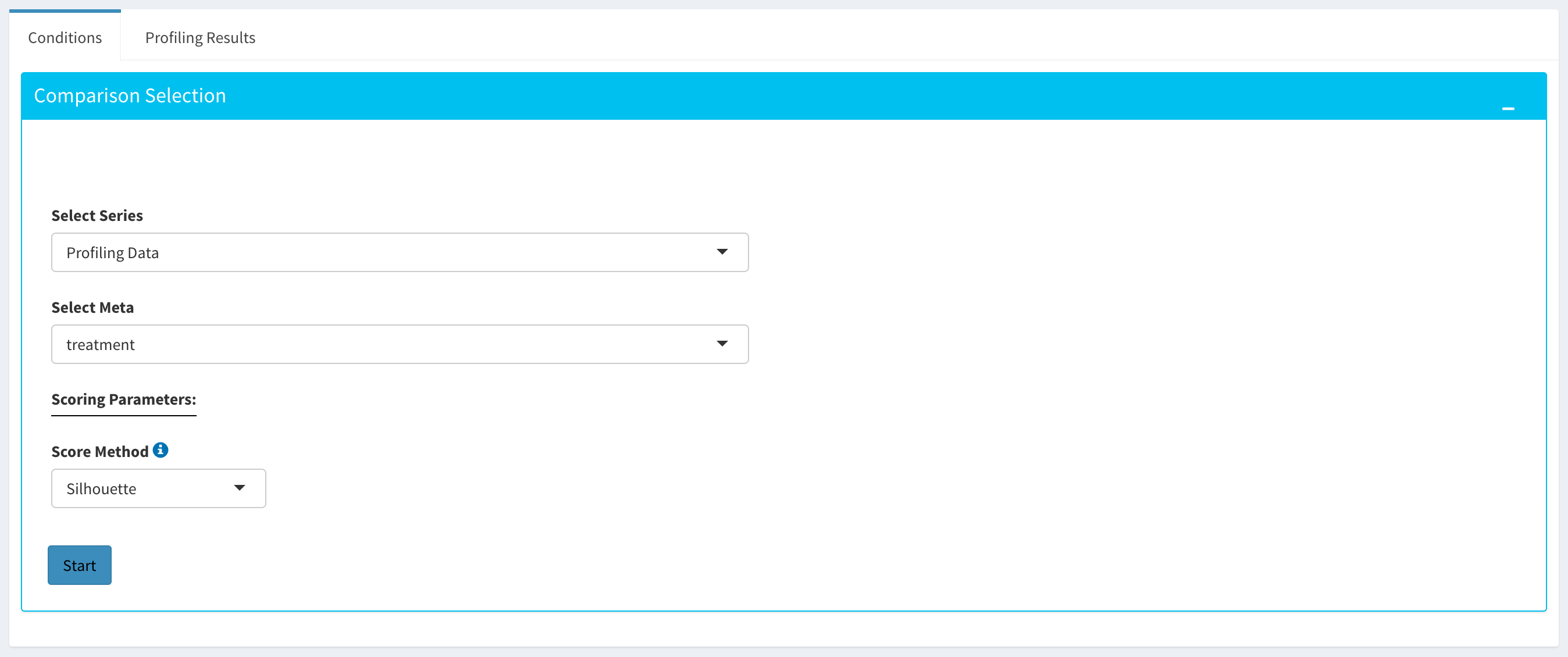
By using the “Comparative Profiling” tab, you can to choose which metadata variables to use as a reference to compare samples and conditions across submitted and reference bulk rna expression datasets. You can select a subset of the data with Select Series option, select a metadata variable with Select Meta option, and choose membership scoring method by Score Method similar to in Computational profiling.

Once you click Start button, Dprofiler calculates the membership scores given conditions/phenotypes in the reference bulk RNA expression data, and visualizes the scores as below.